Local Stochastic Factored Gradient Descent for Distributed Quantum State Tomography

This blog post is about my recent work on distributed quantum state tomography using local stochastic factored gradient descent,¹ published in Control System Letters, IEEE 2023. This is a joint work with my advisors Prof. Tasos Kyrillidis and Prof. Cesar A. Uribe, and my good friend Taha Toghani.

Introduction

Quantum state tomography (QST) is one of the main procedures to identify the nature of imperfections in quantum processing unit (QPU) implementation. For more detailed background on QST, please refer to my previous blog post.

Given the previous blogpost, we will jump directly to the objective function. We again use low-rankness as our prior. That is, we consider the reconstruction of a low-rank density matrix $\rho^\star \in \mathbb{C}^{d \times d}$ on a $n$-qubit Hilbert space, where $d=2^n$, through the following $\ell_2$-norm reconstruction objective: \begin{align} \label{eq:objective} \tag{1} \min_{\rho \in \mathbb{C}^{d \times d}} \quad & f(\rho) := \tfrac{1}{2} ||\mathcal{A}(\rho) - y||_2^2 \\
\text{subject to} \quad& \rho \succeq 0, ~\texttt{rank}(\rho) \leq r. \end{align}

Here, $y \in \mathbb{R}^m$ is the measured data through quantum computer or simulation, and $\mathcal{A}(\cdot): \mathbb{C}^{d \times d} \rightarrow \mathbb{R}^m$ is the linear sensing map. The sensing map relates the density matrix $\rho$ to the measurements through Born rule: $\left( \mathcal{A}(\rho) \right)_i = \text{Tr}(A_i \rho),$ where $A_i \in \mathbb{C}^{d \times d},~i=1, \dots, m$ are the sensing matrices.

One of the motivation for using the low-rank prior is that the sample complexity can be reduced to $O(r \cdot d \cdot \text{poly} \log d)$ from $O(d^2)$.² However, low-rank constraint is a non-convex constraint, which is tricky to handle. To solve \eqref{eq:objective} as is using iterative methods like gradient descent, one needs to perform singular value decomposition on every iteration (in order to project onto the low-rank and PSD subspace), which is prohibitively expensive when $d$ is large, which is almost always the case as $d = 2^n$.

To address that, instead of solving \eqref{eq:objective}, we proposed to solve a factorized version of it, following recent work ³: \begin{align} \label{eq:factored-obj} \tag{2} \min_{U \in \mathbb{C}^{d \times r}} f(UU^\dagger) := \tfrac{1}{2} || \mathcal{A} (UU^\dagger) - y ||_2^2, \end{align} where $U^\dagger$ denotes the adjoint of $U$. Now, \eqref{eq:factored-obj} is an unconstrained problem, and we can use gradient descent on $U$, which iterates as follows:

\begin{align*} \label{eq:fgd} \tag{3} U_{i+1} &= U_{i} - \eta \nabla F(U_k U_k^\dagger) \cdot U_k \\
&= U_k - \eta \left( \frac{1}{m} \sum_{i=1}^m ( \text{Tr}(A_k U_k U_t^\dagger) - y_k ) A_k \right) \cdot U_k \end{align*}

Even though \eqref{eq:factored-obj} is unconstrained and thus we can avoid performing the expensive singular value decomposition on every iteration, $m$ in \eqref{eq:fgd} is still extremely large. In particular, with $r=100$ and $n=30$, the reduced sample complexity still reaches $O\left(r \cdot d \cdot \text{poly}(\log d)\right) \approx 9.65 \times 10^{14}$.

Distributed objective

To handle such explosion of data, We consider the setting where the measurements $y \in \mathbb{R}^m$ and the sensing matrices $\mathcal{A}: \mathbb{C}^{d\times d} \rightarrow \mathbb{R}^m$ from a central quantum computer are locally stored across $M$ different classical machines. These classical machines perform some local operations based on their local data, and communicate back and forth with the central quantum server. Mathematically, we can write the distributed objective as: \begin{align} \label{eq:dist-obj} \tag{4} \min_{U \in \mathbb{C}^{d \times r}} g(U) &= \frac{1}{M} \sum_{i=1}^M g_i(U), \\
\text{where} \quad g_i(U) &:= \mathbb{E}_{j \sim \mathcal{D}_i} ||\mathcal{A}_i^j (UU^\dagger) - y_i^j ||_2^2. \end{align}

We illustrate the above objective with the figure bellow:

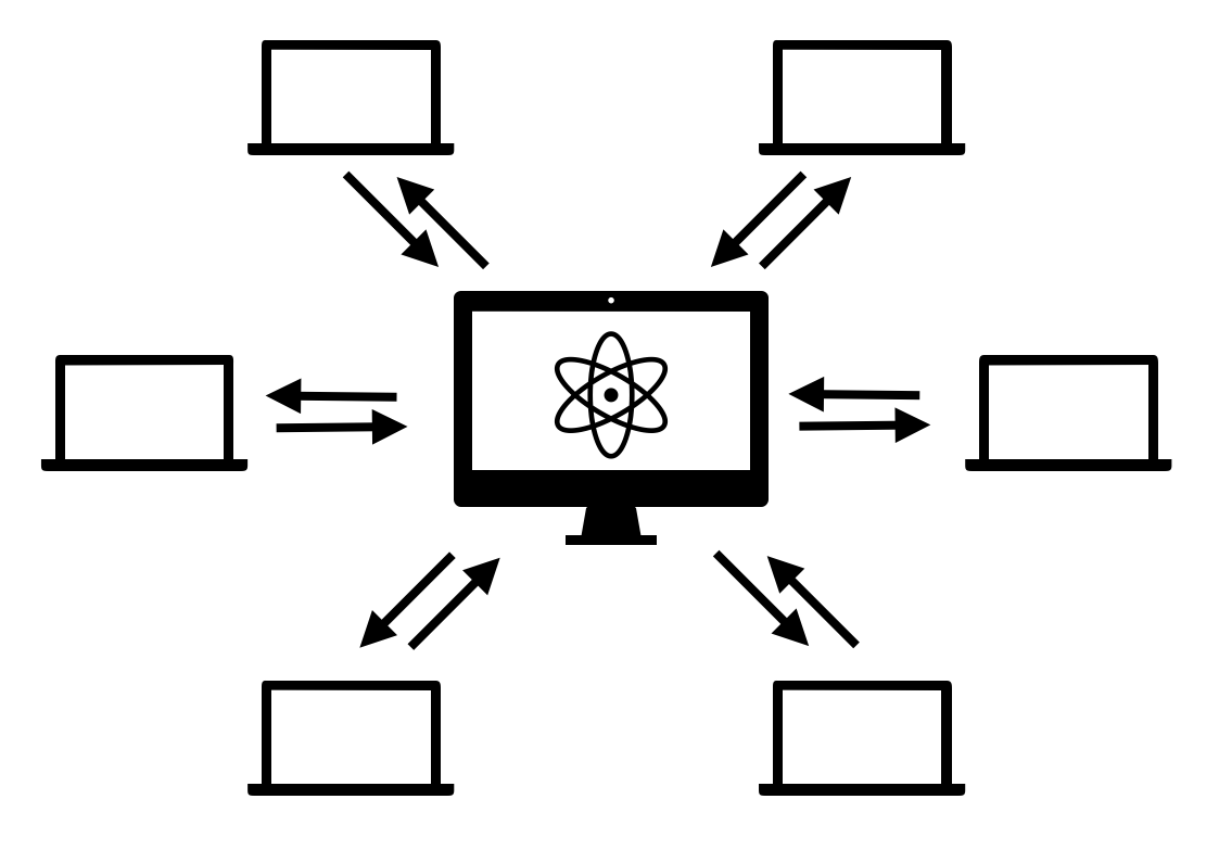
That is, $i$-th machine has sensing matrices $\mathcal{A}_i: \mathbb{C}^{d\times d} \rightarrow \mathbb{R}^{m_i}$ and measurement data $y_i \in \mathbb{R}^{m_i}$, such that the collection of $\mathcal{A}_i$ and $y_i$ for $i \in [M]$ recover the original $\mathcal{A}$ and $y$.

Distributed algorithm

A naive way to implement a distributed algorithm to solve \eqref{eq:dist-obj} is as follows:

• Each machine can take a (stochastic) gradient step: \begin{align} U_k^i = U_{k-1}^i - \eta_{t-1} \nabla g_i^{j_{t-1}} (U_{t-1}^i) \end{align}
• Central quantum server receives next iterate for all $i$ and take average: \begin{align} U_k^i = U_{k-1}^i - \eta_{t-1} \nabla g_i^{j_{t-1}} (U_{t-1}^i) \end{align}

However, such intra-node communication is much more —typically 3-4 order of magnitude more— expensive than inter-node computation.⁴ Therefore, it’s desirable to communicate as little as possible. One way to do so is by performing local iterations on each machine, and communicate only once in a while. We propose the Local Stochastic Factored Gradient Descent (Local SFGD) in the below pseudocode:

The initialization scheme in line 1 (or Eq. (7)) is an adaptation of Theorem 11⁵ to the distributed setting, and is crucial in theory to prove global convergence (however, in practice, we observe thant random intialization also works well). Also notice that there are some pre-defined synchronization (or communication) steps $t_p$, for some $p \in \mathbb{N}$. The algorithm proceeds by, at each time step $t$, a stochastic FGD step is taken in parallel for each machine. Only if the time step equals a pre-defined synchronization step, the local iterates are sent to the server and their average is computed. The average is fed back to each machine, and the process repeats until the time step reaches user-input $T$.

Theoretical guarantees

We will not get into the details of the theoretical guarantees of Local SFGD in this post. Please refer to the paper for more detailed discussion.

That being said, we first introduce the assumptions on the function class and on the stochastic gradients:

Assumption 1 is the standard strong-convexity and $L$-smoothness assumptions, but are restricted (i.e., weaker) in the sense that they only need to hold for PSD matrices. Assumption 2 is quite standard on stochastic-optimization literature.

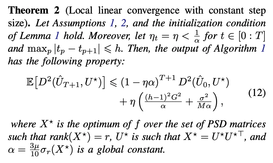
Based on the above assumptions, we prove two results: local linear convergence with a constant step-size (Theorem 2), and local sub-linear conveergence with diminishing step-sizes (Theorem 4). Here, “local convergence” means that the convergence depends on the initialization.

Some remarks to make:

• the last variance term, $\frac{\sigma^2}{M \alpha}$, also shows up in the convergence analysis of SFGD is reduced by the number of machines $M$;
• we assume a single-batch is used in the proof; by using batch size $b > 1$, this term can be further divided by $b$;
• by plugging in $h = 1$ (i.e., synchronization happens on every iteration), the first variance term disappears, exhibiting similar local linear convergence to SFGD.⁶

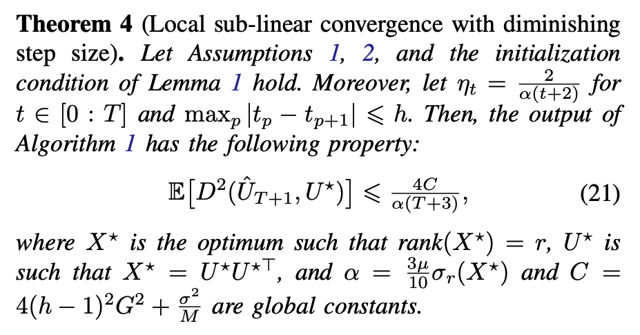
The main message of Theorem 4 is that, by using appropriately diminishing step-sizes, we can achieve local convergence (without any variance term), at the cost of slowing down the convergence rate to a sub-linear one.

Numerical simulations

We use the Local SFGD to reconstruct the Greenberger-Horne-Zeilinger (GHZ) state, using simulated measurement data from Qiskit. GHZ state is known as maximally entangled quantum state, meaning that it exhibits the maximal inter-particle correlation, which does not exist in the classical mechanics. We are interested in: $(i)$ how the number of local steps affect the accuracy defined as $ \varepsilon = || \hat{U}_t \hat{U}_t^\top - \rho^\star ||_F^2,$ where $\rho^\star = U^\star U^{\star \dagger}$ is the true density matrix for the GHZ state; and $(ii)$ the scalability of the distributed setup for various number of classical machines $M$.

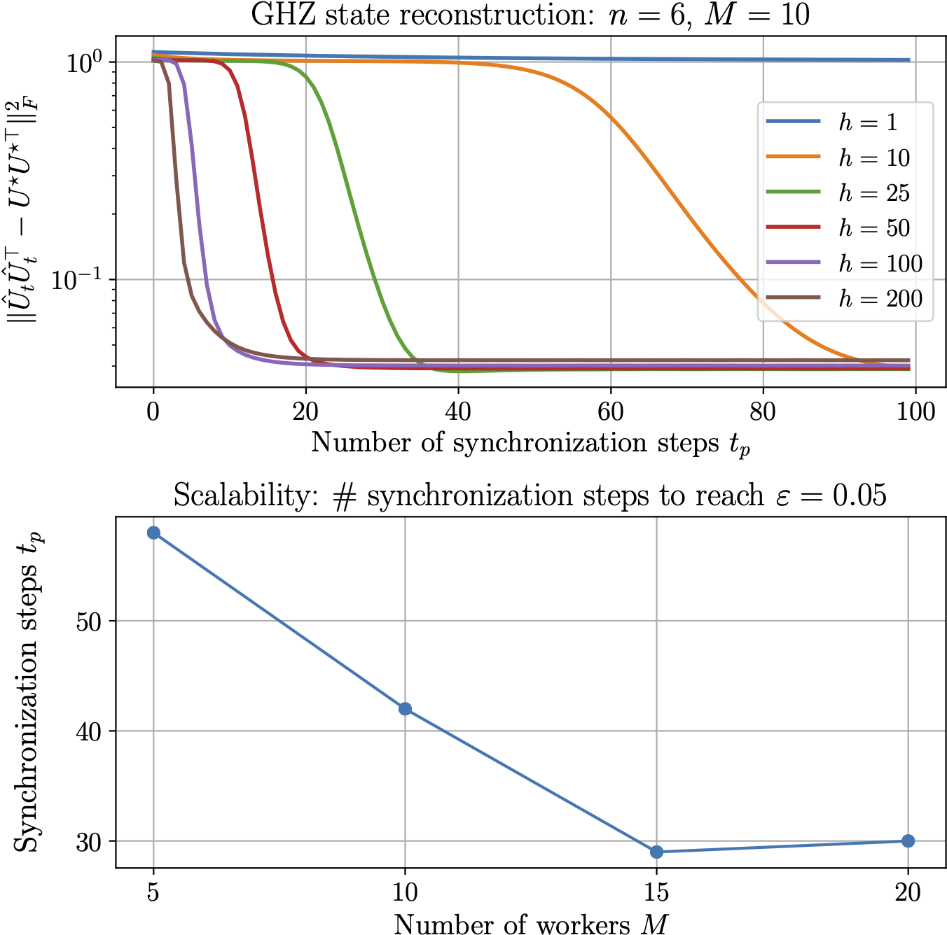
In the top panel of the above plot, we first fix the number of machines $M = 10$ and the number of total synchronization steps to be $100$, and vary the number of local iterations between two synchronization steps, i.e., $h \in {1, 10, 25, 50, 100, 200}.$ We use constant step size $\eta=1$ for all $h$.

Increasing $h$, i.e., each distributed machine performing more local iterations, leads to faster convergence in terms of the synchronization steps. Notably, the speed up gets marginal: e.g., there is not much difference between $h=100$ and $h=200$, indicating there is an ``optimal'' $h$ that leads to the biggest reduction in the number of synchronization steps. Finally, note that $\varepsilon$ does not decrease below certain level due to the inherent finite sampling error of quantum measurements.

In the bottom panel, we plot the number of synchronization steps to reach $\varepsilon \leq 0.05,$ while fixing % the number of local iterations, i.e., $h=20$. We vary the number of workers $M \in {5, 10, 15, 20}$, where each machine gets $200$ measurements. There is a significant speed up from $M=5$ to $M=15$, while for $M=20,$ it took one more syncrhonization step compared to $M=15,$ which is likely due to the stochasticity of SFGD within each machine.

---

1. J. L. Kim, M. T. Toghani, C. A. Uribe and A. Kyrillidis. Local Stochastic Factored Gradient Descent for Distributed Quantum State Tomography. IEEE Control Systems Letters, vol. 7, pp. 199-204, 2023. ↩︎

2. D. Gross, Y.-K. Liu, S. Flammia, S. Becker, and J. Eisert. Quantum state tomography via compressed sensing. Physical review letters, 105(15):150401, 2010. ↩︎

3. A. Kyrillidis, A. Kalev, D. Park, S. Bhojanapalli, C. Caramanis, and S. Sanghavi. Provable quantum state tomography via non-convex methods. npj Quantum Information, 4(36), 2018. ↩︎

4. Guanghui Lan, Soomin Lee, and Yi Zhou. Communication-efficient algorithms for decentralized and stochastic optimization. Mathematical Programming 180.1-2. 237-284. 2020. ↩︎

5. S. Bhojanapalli, A. Kyrillidis, S. Sanghavi. Dropping Convexity for Faster Semi-definite Optimization. 29th Annual Conference on Learning Theory, in Proceedings of Machine Learning Research. 49:530-582. 2016. ↩︎

6. J. Zeng, K. Ma, and Y. Yao. “On global linear convergence in stochastic nonconvex optimization for semidefinite programming.” IEEE Transactions on Signal Processing 67.16. 4261-4275. 2019, ↩︎