Convergence and Stability of the Stochastic Proximal Point Algorithm with Momentum

Introduction

In this blog post, I will introduce the stochastic proximal point algorithm with momentum (SPPAM) based on this paper,¹ which is forthcoming in Learning for Dynamics and Control (L4DC) 2022.

Background

We focus on unconstrained empirical risk minimization: \begin{align} \label{eq:obj} \tag{1} \min_{x \in \mathbb{R}^p} ~f(x) = \frac{1}{n} \sum_{i=1}^n f_i(x). \end{align}

Stochastic gradient descent (SGD) has become the de facto method to solve \eqref{eq:obj} used by the machine learning community, mainly due to its computational efficiency. SGD iterates as follows: \begin{align} \label{eq:sgd} \tag{2} x_{t+1} = x_t - \eta \nabla f_{i_t}(x_t), \end{align} where $\eta$ is the step size, and $\nabla f_i$ is the (stochastic) gradient computed at the $i$-th data point.

While computationally efficient, SGD in \eqref{eq:sgd} suffers from two major limitations: $(i)$ slow convergence, and $(ii)$ numerical instability. Due to the (stochastic) gradient noise, SGD could take longer to converge in terms of iterations. Moreover, SGD suffers from numerical instabilities both in theory and practice, allowing only a small range of $\eta$ values that lead to convergence, which often depend on unknown quantities. ^{2 3}

Acceleration via Momentum.

With respect to the slow convergence, many variants of accelerated methods have been proposed, including the Polyak’s momentum ⁴ and the Nesterov’s acceleration ⁵ methods. These methods allow faster (sometimes optimal) convergence rates, while having virtually the same computational cost as SGD. In particular, SGD with momentum (SGDM) iterates as follows: \begin{align} \label{eq:sgdm} \tag{3} x_{t+1} = x_t - \eta \nabla f_{i_t}(x_t) + \beta (x_t - x_{t-1}), \end{align} where $\beta \in [0,1)$ is the momentum parameter. The intuition is that, if the direction from $x_{t-1}$ to $x_t$ was “correct,” then SGDM utilizes this inertia weighted by the momentum parameter $\beta,$ instead of just relying on the current point $x_t.$

Yet, SGDM could be hard to tune: SGDM adds another hyperparameter—momentum $\beta$—to an already sensitive stochastic procedure of SGD. As such, various works have found that such motions could aggravate the instability of SGD. ^{6 7 8}

Stability via Proximal Updates.

With respect to the numerical stability, variants of SGD that utilize proximal updates have recently been proposed. The proximal point algorithm (PPA) obtains the next iterate for minimizing $f$ by solving the following optimization problem: \begin{align} \label{eq:ppa} \tag{6} x_{t+1} = \arg \min_{x\in \mathbb{R}^p} \left\{ f(x) + \tfrac{1}{2\eta} || x - x_t ||_2^2 \right\}, \end{align} which is equivalent to implicit gradient descent (IGD) by the first-order optimality condition: \begin{align} \label{eq:igd} \tag{7} x_{t+1} = x_t - \eta \nabla f(x_{t+1}). \end{align} In words, instead of minimizing $f$ directly, PPA minimizes $f$ with an additional quadratic term. This small change brings a major advantage to PPA: if $f$ is convex, the added quadratic term can make the problem strongly convex; if $f$ is non-convex, PPA can make it convex.

Thanks to this conditioning property, PPA exhibits different behavior compared to GD in the deterministic setting. For a convex function $f$, PPA satisfies: ⁹ \begin{align} \label{eq:ppm-conv-rate-guller} \tag{8} f(x_T) - f(x^\star) \leq O \left( \tfrac{1}{\sum_{t=1}^T \eta_t} \right),
\end{align} after $T$ iterations. By setting the step size $\eta_t$ to be large, PPA can converge ``arbitrarily'' fast.

Due to this remarkable property, PPA was soon considered in the stochastic setting, dubbed as stochastic proximal iterations (SPI) ^{10 11} or implicit SGD ^{12 13}. These works generally indicate that, in the asymptotic regime, SGD and SPI/ISGD have the same convergence behavior; but in the non-asymptotic regime, SPI/ISGD outperforms SGD due to numerical stability provided by utilizing proximal updates.

Our Approach: Stochastic PPA with Momentum (SPPAM).

The main question we wanted to answer in this work was as follows: $$\text{Can we accelerate stochastic PPA while preserving its numerical stability?}$$

SPPAM iterates as follows: \begin{align} x_{t+1} &= x_t - \eta \left (\nabla f(x_{t+1}) + \varepsilon_{t+1}\right) + \beta (x_t - x_{t-1}) \label{eq:acc-stoc-ppa}. \tag{5} \end{align}

Apart from the similarity between SPPAM in \eqref{eq:acc-stoc-ppa} and SGDM in \eqref{eq:sgdm}, SPPAM shares the same geometric intuition as Polyak’s momentum for SGDM. Disregarding the stochastic errors, the update in \eqref{eq:acc-stoc-ppa} follows from the solution of: \begin{align*} \arg \min_{x \in \mathbb{R}^p} \left\{ f(x) + \tfrac{1}{2\eta} ||x-x_t||_2^2 - \tfrac{\beta}{\eta} \langle x_t - x_{t-1}, x \rangle \right\}. \end{align*}

We can get a sense of the behavior of SPPAM from this expression. First, for large $\eta$, the algorithm is minimizing the original $f.$ For small $\eta$, the algorithm not only tries to stay local by minimizing the quadratic term, but also tries to minimize $-\frac{\beta}{\eta} \langle x_t - x_{t-1}, x \rangle$. By the definition of inner product, this means that $x$, on top of minimizing $f$ and staying close to $x_t$, also tries to move along the direction from $x_{t-1}$ to $x_t$. This intuition aligns with that of Polyak’s momentum.

The quadratic model case

For simplicity, we first consider the convex quadratic optimization problem under the deterministic setting. Specifically, we consider the objective function: \begin{align} \label{eq:obj-quad} \tag{10} f(x) = \frac{1}{2} x^\top A x - b^\top x, \end{align} where $A \in \mathbb{R}^{p\times p}$ is positive semi-definite with eigenvalues $\left[ \lambda_1, \dots, \lambda_p \right]$. Under this scenario, we can study how the step size $\eta$ and the momentum $\beta$ affect each other, by deriving exact conditions that lead to convergence for each algorithm. The comparison list includes gradient descent (GD), gradient descent with momentum (GDM), the PPA, and PPA with momentum (PPAM).

Proposition 1 (GD)¹⁴ To minimize \eqref{eq:obj-quad} with gradient descent, the step size $\eta$ needs to satisfy $0 < \eta < \frac{2}{\lambda_i}~~\forall i$, where $\lambda_i$ is the $i$-th eigenvalue of $A$.

Proposition 2 (PPA)¹ To minimize \eqref{eq:obj-quad} with PPA, the step size $\eta$ needs to satisfy $\left| \frac{1}{1+\eta \lambda_i} \right| < 1~~\forall i$.

Proposition 3 (GDM)¹⁴ To minimize \eqref{eq:obj-quad} with gradient descent with momentum, the step size $\eta$ needs to satisfy $0 < \eta \lambda_i < 2 + 2\beta$ ~ $\forall i$, where $0 \leq \beta < 1.$

Proposition 4 (PPAM)¹ Let $\delta_i = \left( \frac{\beta+1}{1+\eta \lambda_i} \right)^2 - \frac{4\beta}{1+\eta \lambda_i}.$ To minimize \eqref{eq:obj-quad} with PPAM, the step size $\eta$ and momentum $\beta$ need to satisfy $~\forall i$:

• $\eta > \frac{\beta-1}{\lambda_i},\quad$ if $\delta_i \leq 0$;
• $\frac{\beta+1}{1+\eta \lambda_i} + \sqrt{\delta_i} < 2,\quad$ if $\delta_i > 0$ and $\frac{\beta+1}{1+\eta \lambda_i} \geq 0$;
• $\frac{\beta+1}{1+\eta \lambda_i} - \sqrt{\delta_i} > -2,\quad$ otherwise.

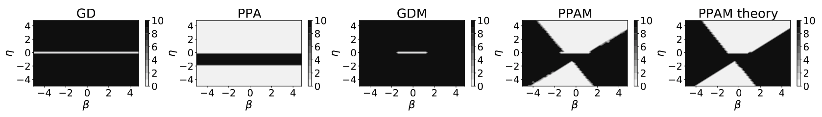
Given the above propositions, we can study the stability with respect to the step size $\eta$ and the momentum $\beta$ for the considered algorithms. Numerical simulations support the above propositions, and are illustrated in the above figure, matching the theoretical conditions exhibited above.

In particular, for GD, only a small range of step sizes $\eta$ leads to convergence (small white band); this “white band” corresponds to the restriction that $\eta$ has to satisfy $\eta < \tfrac{2}{\lambda_i}$ for all $i$. On the other hand, PPA/IGD converges in much wider choices of $\eta$; this is apparent from Proposition 2, since $\left| \frac{1}{1+\eta \lambda_i} \right|$ can be arbitrarily small for larger values of $\eta$. GDM requires both $\eta$ and $\beta$ to be in a small region to converge, following Proposition 3. Finally, PPAM converges in much wider choices of $\eta$ and $\beta$; e.g., the conditions in Proposition 4 define different regions of the pair $(\eta, \beta)$ that lead to convergence, some of which set both $\eta$ and $\beta$ to be negative. Note that the empirical convergence region of PPAM almost exactly matches the theoretical region that leads to convergence in Proposition 4.

In the next section, we will see how this pattern translates to a general strongly convex function $f,$ with stochasticity.

Main Results

In this section, we theoretically characterize the convergence and stability behavior of SPPAM.

We follow the stochastic errors of PPA, as set up in this paper.¹³ We can then express \eqref{eq:acc-stoc-ppa} as: \begin{align*} x_{t+1}^+ &= x_t - \eta \nabla f(x_{t+1}^+) + \beta (x_t - x_{t-1}) \\
x_{t+1} &= x_{t+1}^+ - \eta \varepsilon_{t+1}. \end{align*}

Note that $x_{t+1}^+$ is an auxiliary intermediate variable that is used for the analysis only.

We further assume the following:

Assumption 1 $f$ is a $\mu$-strongly convex function: for some fixed $\mu > 0$ and for all $x$ and $y$, \begin{align*} \langle \nabla f(x)-\nabla f(y), x - y \rangle \geq \mu ||x-y ||_2^2. \end{align*}

Assumption 2 There exists fixed $\sigma^2 > 0$ such that, given the natural filtration $\mathcal{F}_{t-1},$ \begin{align*} \mathbb{E}\left[ \varepsilon_t \mid \mathcal{F}_{t-1} \right] = 0 \quad\text{and}\quad \mathbb{E}\left[ | \varepsilon_t \mid \mathcal{F}_{t-1} |^2 \right] \leq \sigma^2 \quad\text{for all}\quad t. \end{align*}

Is SPPAM faster than SPPA?

We first study whether SPPAM enjoys faster convergence than SPPA. We start with the iteration invariant bound, which expresses the expected error at $x_{t+1}$ in terms of its previous iterates:

Theorem 5 For $\mu$-strongly convex $f(\cdot)$, SPPAM satisfies the following iteration invariant bound: \begin{align} \label{eq:onestep-acc-stoc-prox} \tag{11} \mathbb{E} \big[ || x_{t+1 }- x^\star ||_2^2 \big] &\leq \tfrac{4}{(1+\eta \mu)^2} \mathbb{E} \big[ ||x_t - x^\star ||_2^2 \big] \\
&\quad+ \tfrac{4\beta^2}{(1+\eta \mu)^2\left( 4-(1+\beta)^2 \right)} \mathbb{E} \big[ ||x_{t-1} - x^\star ||_2^2 \big] + \eta^2 \sigma^2. \end{align}

Notice that all terms –except the last one– are divided by $(1+\eta \mu)^2.$ Thus, large step sizes $\eta$ help convergence (to a neighborhood), reminiscent of the convergence behavior of PPA in \eqref{eq:ppm-conv-rate-guller}.

Based on \eqref{eq:onestep-acc-stoc-prox}, we can write the following $2\times 2$ system that characterizes the progress of SPPAM: \begin{align} \label{eq:two-by-two-onestep} \tag{12} \begin{bmatrix} \mathbb{E} \big[ ||x_{t+1} - x^\star ||_2^2 \big] \\
\mathbb{E} \big[ ||x_t - x^\star ||_2^2 \big] \end{bmatrix} &\leq A \cdot \begin{bmatrix} \mathbb{E} \big[ ||x_t - x^\star ||_2^2 \big] \\
\mathbb{E} \big[ ||x_{t-1} - x^\star ||_2^2 \big] \end{bmatrix} + \begin{bmatrix} \eta^2 \sigma^2 \\
0 \end{bmatrix}, \end{align}

where $A = \begin{bmatrix} \frac{4}{(1+\eta \mu)^2} & \frac{4\beta^2}{(1+\eta \mu)^2\left( 4-(1+\beta)^2 \right)} \\
1 & 0 \end{bmatrix}$. It is clear that the spectrum of the contraction matrix $A$ determines the convergence rate to a neighborhood. This is summarized in the following lemma:

Lemma 6 The maximum eigenvalue of $A$, which determines the convergence rate of SPPAM, is: \begin{align} \label{eq:acc-stoc-ppa-conv-rate} \tag{13} \tfrac{2}{(1+\eta \mu)^2} + \sqrt{ \tfrac{4}{(1+\eta \mu)^4} + \tfrac{4\beta^2}{(1+\eta \mu)^2(4 - (1+\beta)^2)}}. \end{align}

Notice the one-step contraction factor in \eqref{eq:acc-stoc-ppa-conv-rate} is of order $O(1/\eta^2),$ exhibiting acceleration compared to that of SPPA for strongly convex objectives: $1/(1+2\eta \mu) \approx O(1/\eta).$¹³

However, due to the additional terms, it is not immediately obvious when SPPAM enjoys faster convergence than SPPA. We thus characterize this condition more precisely in the following corollary:

Corollary 7 For $\mu$-strongly convex $f$, SPPAM enjoys better contraction factor than SPPA if: \begin{align*} \frac{4\beta^2}{4 - (1+\beta)^2} < \frac{\eta^2 \mu^2 - 6\eta\mu - 3}{(1+\eta \mu)^2}. \end{align*}

In words, for a fixed step size $\eta$ and given a strongly convex parameter $\mu$, there is a range of momentum parameters $\beta$ that exhibits acceleration compared to SPPA.

In contrast to (stochastic) gradient method analyses in convex optimization, where acceleration is usually shown by improving the dependency on the condition number from $\kappa = \tfrac{L}{\mu}$ to $\sqrt{\kappa},$ such a claim can hardly be made for stochastic proximal point methods. This is also the case in deterministic setting, where (Nesterov’s) accelerated PPA converges for strongly convex $f$ as in:¹⁵ \begin{align} f(x_T) - f(x^\star) \leq O \left( \frac{1}{ \big( \sum_{t=1}^T \sqrt{\eta_t} \big)^2} \right), \label{eq:ppm-acc-conv-rate-guller} \tag{14} \end{align} which is faster than the rate in \eqref{eq:ppm-conv-rate-guller}.

As shown in Theorem 5, our convergence analysis of SPPAM does not depend on $L$-smoothness at all. This robustness of SPPAM is also confirmed in numerical simulations in the next section, where SPPAM exhibits the fastest convergence rate, virtually independent of the different settings considered.

Is SPPAM more stable than SGDM?

Theorem 9 For $\mu$-strongly convex $f$, assume SPPAM is initialized with $x_0 = x_{-1}$. Then, after $T$ iterations, we have: \begin{align} \label{eq:Tstep-acc-stoc-prox} \tag{15} &\mathbb{E} \big[ ||x_T - x^\star ||_2^2 \big] \leq \frac{2 \sigma_1^T}{\sigma_1 - \sigma_2} % \left( \left( ||x_0-x^\star ||_2^2 + \tfrac{\eta^2 \sigma^2}{1-\theta}\right) \cdot (1+\theta) \right)
+ \frac{\eta^2 \sigma^2}{1-\theta}, \end{align} where $\theta=\frac{4}{(1+\eta\mu)^2} + \tfrac{4\beta^2}{(1+\eta\mu)^2(4-(1+\beta)^2)}.$

Here, $\sigma_{1, 2}$ are the eigenvalues of $A$, and \begin{align} \label{eq:discount-init} \tag{16} \tfrac{2 \sigma_1^T}{\sigma_1 - \sigma_2} = \tau^{-1} \cdot \left( \tfrac{2}{(1+\eta\mu)^2} + \tau \right)^T \quad \text{with} \quad \tau = \sqrt{ \tfrac{4}{(1+\eta \mu)^4} + \tfrac{4\beta^2}{(1+\eta \mu)^2(4 - (1+\beta)^2)}}. \end{align}

The above theorem states that the term in \eqref{eq:discount-init} determines the discounting rate of the initial conditions. In particular, the condition that leads to an exponential discount of the initial conditions is characterized by the following theorem:

Theorem 10 Let the following condition hold: \begin{align} \label{eq:init-discount-condition} \tag{17} % \left( \frac{1-\beta}{1+2 \eta \mu} \right)^2 + \frac{\beta^2}{1+2\eta \mu} \left( \frac{2-\beta}{2-\beta(1+\beta)} \right) < \frac{1}{4}. \tau = \sqrt{ \tfrac{4}{(1+\eta \mu)^4} + \tfrac{4\beta^2}{(1+\eta \mu)^2(4 - (1+\beta)^2)}} < \tfrac{1}{2}. \end{align} Then, for $\mu$-strongly convex $f$, initial conditions of SPPAM exponentially discount: i.e., in \eqref{eq:Tstep-acc-stoc-prox},
\begin{align*} \tfrac{2 \sigma_1^T}{\sigma_1 - \sigma_2} = \tau^{-1} \cdot \left( \tfrac{2}{(1+\eta\mu)^2} + \tau \right)^T =C^T, \quad\text{where}\quad C \in (0, 1). \end{align*}

To provide more context of the condition in Theorem 10, we make an ``unfair" comparison of \eqref{eq:init-discount-condition}, which holds for general strongly convex $f,$ to the condition that accelerated SGD requires for strongly convex quadratic objective in \eqref{eq:obj-quad}.

This paper shows that Nesterov’s accelerated SGD converges to a neighborhood at a linear rate for strongly convex quadratic objective if $\max{ \rho_\mu(\eta, \beta),~\rho_L(\eta, \beta) } < 1$, where $\rho_\lambda(\eta, \beta)$ for $\lambda \in {\mu, L}$ is defined as: \begin{align} \label{eq:sgdm-spectral-rad} \rho_\lambda(\eta, \beta) = \begin{cases} \frac{|(1+\beta)(1-\eta \lambda)|}{2} + \frac{\sqrt{\Delta_\lambda}}{2} & \text{if}~\Delta_\lambda \geq 0, \
\sqrt{\beta (1-\eta \lambda)} & \text{otherwise}, \end{cases} \end{align} with $\Delta_\lambda = (1+\beta)^2 (1-\eta \lambda)^2 - 4\beta(1-\eta \lambda)$. This condition for convergence can thus be divided into three cases, depending on the range of $\eta \lambda$. Define $\psi_{\beta, \eta, \lambda} = (1 + \beta)(1 - \eta \lambda)$. Then: \begin{align*} \begin{cases} \eta \lambda \geq 1, & \text{Converges if }-\psi_{\beta, \eta, \lambda} + \sqrt{\Delta_\lambda} < 2, \\ \frac{(1-\beta)^2}{(1+\beta)^2} \leq \eta \lambda < 1, & \text{Always converges}, \\
\eta \lambda < \frac{(1-\beta)^2}{(1+\beta)^2}, &\text{Converges if }\psi_{\beta, \eta, \lambda} + \sqrt{\Delta_\lambda}< 2 . \end{cases} \end{align*}

Now, consider the standard momentum value $\beta = 0.9.$ For the first case, the convergence requirement translates to $1 \leq \eta \lambda \leq \tfrac{24}{19}.$ The second range is given by $\frac{1}{361} \leq \eta \lambda < 1$. The third condition is lower bounded by 2 for $\beta=0.9,$ leading to divergence. Combining, accelerated SGD requires $0.0028 \approx \frac{1}{361} \leq \eta \lambda \leq \frac{24}{19} \approx 1.26$ to converge for strongly convex quadratic objectives, set aside that this bound has to satisfy for (unknown) $\mu$ or $L$. Albeit an unfair comparison, for general strongly convex objective, \eqref{eq:init-discount-condition} becomes $\eta \mu > 4.81$ for $\beta=0.9.$ Even though $\mu$ is unknown, one can see this condition is easy to satisfy, by using a sufficiently large step size $\eta$.

Experiments

In this section, we perform numerical experiments to study the convergence behaviors of SPPAM, SPPA, SGDM, and SGD, using generalized linear models (GLM).

GLM subsumes a wide family of models including linear, logistic, and Poisson regressions. Different models connects the linear predictor $\gamma=\langle a_i, x^\star \rangle$ through different \textit{mean} functions $h(\cdot)$. We focus on linear and Poisson regression models, where mean functions are defined respectively as $h(\gamma) = \gamma$ and $h(\gamma) = e^\gamma$. The former is an “easy” case, where objective is strongly convex, satisfying Assumption 1. The latter is a “hard” case with non-Lipschitz continuous gradients, where SGD and SGDM are expected to suffer.

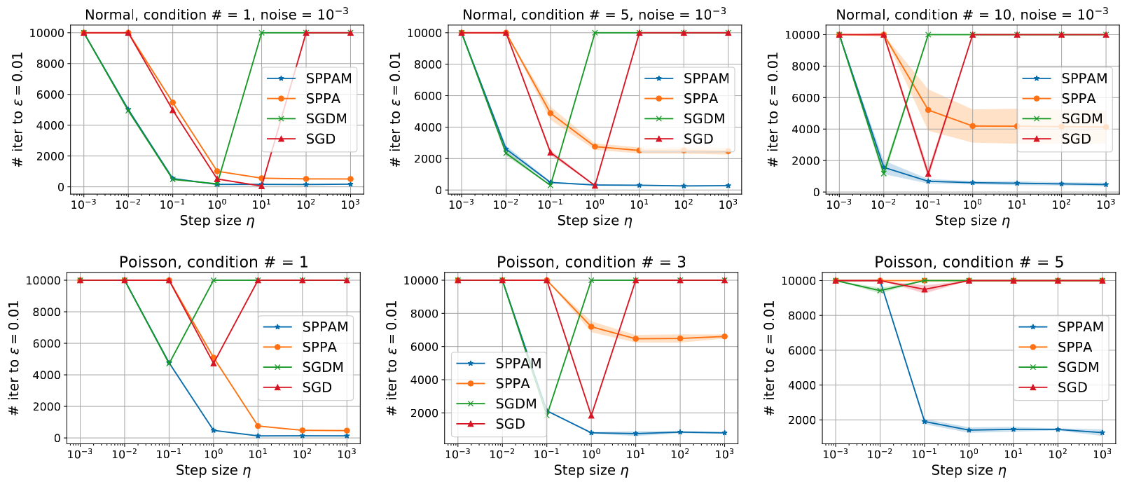
In the top row of above figure, we present the results for the linear regression with different condition numbers, with gaussian noise level $\texttt{1e-3}$. We run each algorithm constant step size $\eta$ varying from $10^{-3}$ to $10^3$ with $10\times$ increment, and with $\beta=0.9$. As expected, SGD and SGDM only converge for specific step size $\eta$, while SPPA and SPPAM converge for much wider ranges. In terms of convergence rate, SPPAM converges faster than SPPA in all scenarios, which improves or matches the rate of SGDM, when it converges. As $\kappa$ increases, the range of $\eta$ that leads to convergence for SGD and SGDM shrinks; notice the sharper “$\lor$” shape for SGD and SGDM for $\kappa = 10$ (3rd), compared to $\kappa=5$ (2nd) or $\kappa=1$ (1st). SPPA also slightly slows down as $\kappa$ increases, while SPPAM converges essentially in the same manner for all scenarios.

Such trend is much more pronounced for the Poisson regression case presented in the bottom row. Due to the exponential mean function $h(\cdot)$ for Poisson model, the outcomes are extremely sensitive, and its likelihood does not satisfy standard assumptions like $L$-smoothness. As such, SGD and SGDM struggles with slow convergence even when $\kappa = 1$ (1st), while also exhibiting instability—each method converges only for a single choice of $\eta$ considered. Similar trend is shown when $\kappa=3$ (2nd) where SPPA starts slowing down. For $\kappa = 5$ (3rd), all methods except for SPPAM did not make much progress in $10^4$ iterations, for the entire range of $\eta$ and $\beta$ considered. Quite remarkably, SPPAM still converges in the same manner without sacrificing both the convergence rate and the range of hyperparameters that lead to convergence.

Conclusion

We propose the stochastic proximal point algorithm with momentum (SPPAM), which directly incorporates Polyak’s momentum inside the proximal step. We show that SPPAM converges to a neighborhood at a faster rate than stochastic proximal point algorithm (SPPA), and characterize the conditions that result in acceleration. Further, we prove linear convergence of SPPAM to a neighborhood, and provide conditions that lead to an exponential discount of the initial conditions, akin to SPPA. We confirm our theory with numerical simulations on linear and Poisson regression models; SPPAM converges for all the step sizes that SPPA converges, with a faster rate that matches or improves SGDM.

---

1. Junhyung Lyle Kim, Panos Toulis, and Anastasios Kyrillidis. Convergence and stability of the stochastic proximal point algorithm with momentum. arXiv preprint arXiv:2111.06171, 2021. ↩︎

2. Eric Moulines and Francis R. Bach. Non-Asymptotic Analysis of Stochastic Approximation Algorithms for Machine Learning. In J. Shawe-Taylor, R. S. Zemel, P. L. Bartlett, F. Pereira, and K. Q. Weinberger, editors, Advances in Neural Information Processing Systems 24, pages 451–459. Curran Associates, Inc., 2011. ↩︎

3. Robert M Gower, Nicolas Loizou, Xun Qian, Alibek Sailanbayev, Egor Shulgin, and Peter Richtarik. SGD: General Analysis and Improved Rates. Proceedings of the 36 th International Conference on Machine Learning, page 10, 2019. ↩︎

4. Boris T Polyak. Some methods of speeding up the convergence of iteration methods. Ussr computational mathematics and mathematical physics, 4(5):1–17, 1964. ↩︎

5. Yurii Nesterov et al. Lectures on convex optimization, volume 137. Springer, 2018. ↩︎

6. Chaoyue Liu and Mikhail Belkin. Accelerating sgd with momentum for over-parameterized learning. arXiv preprint arXiv:1810.13395, 2018. ↩︎

7. Rahul Kidambi, Praneeth Netrapalli, Prateek Jain, and Sham Kakade. On the insufficiency of existing momentum schemes for stochastic optimization. In 2018 Information Theory and Applications Workshop (ITA), pages 1–9. IEEE, 2018. ↩︎

8. Mahmoud Assran and Michael Rabbat. On the Convergence of Nesterov’s Accelerated Gradient Method in Stochastic Settings. Proceedings of the 37 th International Conference on Machine Learning, 2020. ↩︎

9. Osman Guler. On the convergence of the proximal point algorithm for convex minimization. ¨ SIAM journal on control and optimization, 29(2):403–419, 1991. ↩︎

10. Ernest K Ryu and Stephen Boyd. Stochastic Proximal Iteration: A Non-Asymptotic Improvement Upon Stochastic Gradient Descent. Author website, page 42, 2017. ↩︎

11. Hilal Asi and John C Duchi. Stochastic (approximate) proximal point methods: Convergence, optimality, and adaptivity. SIAM Journal on Optimization, 29(3):2257–2290, 2019. ↩︎

12. Panos Toulis and Edoardo M Airoldi. Asymptotic and finite-sample properties of estimators based on stochastic gradients. The Annals of Statistics, 45(4):1694–1727, 2017. ↩︎

13. Panos Toulis, Thibaut Horel, and Edoardo M Airoldi. The proximal robbins–monro method. Journal of the Royal Statistical Society: Series B (Statistical Methodology), 83(1):188–212, 2021. ↩︎

14. Gabriel Goh. Why momentum really works. Distill, 2(4):e6, 2017. ↩︎

15. Osman Guler. New proximal point algorithms for convex minimization. ¨ SIAM Journal on Optimization, 2(4):649–664, 1992. ↩︎